An Excel chart consists of a number of different elements. For example, all charts contain a plot area and at least one data series. A chart can also contain elements such as a chart title, axes, data labels, and so on. To work with a particular chart element, you need to select it — something that is often easier said than done.
Excel provides three ways to select a particular chart element:
- Use the mouse.
- Use the keyboard.
- Use the Chart Elements control.
Selecting with the mouse
To select a chart element with your mouse, just click it. The chart element appears with small circles at the corners.
To ensure that you selected the chart element you intended to select, view the Chart Element control, located in the Chart Tools➜Format➜Current Selection group on the Ribbon.
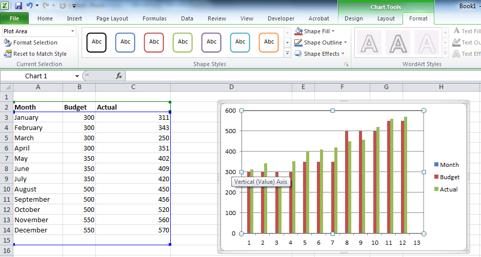
Also, notice that when you move the mouse over a chart, a small chart tip displays the name of the chart element under the mouse pointer. Below shows the Chart Elements control and the tooltip when a chart’s vertical axis is selected.
The Chart Element control displays the name of the selected chart element, and a tooltip also describes the selection. In this example, Vertical (Value) Axis is selected.
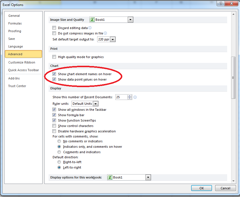
Note: If these chart tips annoy you, you can turn them off. Choose File➜Options and click the Advanced tab in the Excel Options dialog box. Locate the Chart section and deselect either or both of the check boxes labeled Show Chart Element Names On Hover or Show Data Point Values On Hover.
Some chart elements (such as a series, legend, or data label) consist of multiple items. For example, a chart series element is made up of individual data points. To select a particular data point, click twice: First click the series to select it; then click the specific element within the series (such as a column or a line chart marker). Selecting the element enables you to apply formatting to only a particular data point in a series.
You might find that some chart elements are difficult to select with the mouse. If you rely on the mouse for selecting a chart element, you might have to click it several times before the element you want is selected. Fortunately, Excel provides other ways to select a chart element, and it’s worth your while to be familiar with them.
Selecting with the keyboard
When a chart is active, you can use the up-arrow and down-arrow keys on your keyboard to cycle among the chart’s elements. Again, keep your eye on the Chart Elements control, to ensure that the selected chart element is what you think it is.
When a chart series is selected, use the left-arrow and right-arrow keys to select an individual item within the series. Similarly, when a set of data labels is selected, you can select a specific data label by pressing the left-arrow or right-arrow key. And, when a legend is selected, you can select individual elements within the legend by using the left-arrow or right-arrow key.
Selecting with the Chart Element control
The Chart Element control is so useful, that it’s available in three locations:
- In the Chart Tools➜Layout➜Current Selection group of the Ribbon

- In the Chart Tools➜Format➜Current Selection group of the Ribbon

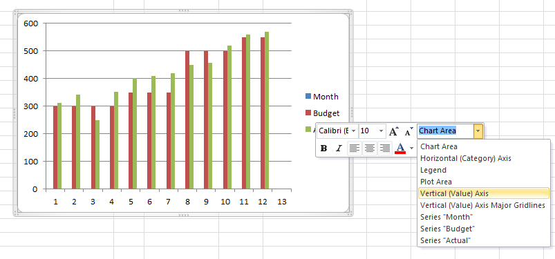
- In the Mini Toolbar that appears when you right-click a chart element This control displays the name of the selected chart element. Because it’s a drop-down control, you can also use it to select a particular element in the active chart. Below Figure shows the Chart Element control in the Mini Toolbar.
This control lists only the top-level elements in the chart. To select an individual data point within a series, for example, you need to select the series and then use the left and right arrow keys (or your mouse) to select the data point.
Note: When a single data point is selected, the Chart Element control will display the name of the selected element, even though it’s not available for selection in the drop-down list.
If you do a lot of work with charts, you might want to add the Chart Element to yet another location: your Quick Access toolbar. That way, it’s always visible regardless of which Ribbon tab is selected. To add the control to your Quick Access toolbar, right-click the down-arrow in the control, and choose Add to Quick Access Toolbar.


