You might be familiar with Excel’s PivotTable feature, which creates a summary table from a list. But what if you want to perform the opposite operation? This tip describes how to create a list from a simple two-variable summary table.
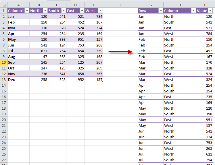
The worksheet shown in Figure 167-1 shows the type of transformation I’m talking about. Range A1:E13 contains the original summary table: 48 data points. Columns G:I show part of a 48-row table derived from the summary table. In other words, every value in the original summary table is converted to a row, which also contains the value’s corresponding product name and month.
This type of list is useful because it can be sorted and manipulated in other ways.
Figure 167-1: Converting a summary table to a list.
The trick to creating this reverse pivot table is to use a pivot table. But before you can make use of this technique, you must add the PivotTable Wizard command to your Quick Access toolbar.
Excel 2007 and Excel 2010 still support the PivotTable Wizard, but it’s not available on the Ribbon. To gain access to the PivotTable Wizard, follow these steps:
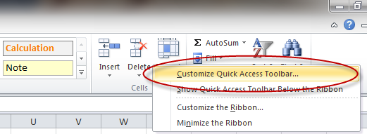
1. Right-click the Quick Access toolbar and choose Customize Quick Access Toolbar from the shortcut menu.
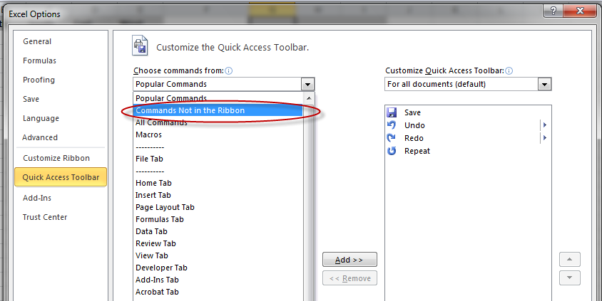
2. On the Quick Access Toolbar tab of the Excel Options dialog box, choose Commands Not in the Ribbon from the drop-down list on the left.
3. Scroll down the list and select PivotTable and PivotChart Wizard from the list.

4. Click Add.
5. Click OK to close the Excel Options dialog box.
After you perform these steps, your Quick Access toolbar displays a new icon.
Now it’s time to convert the summary table to a list. Keep in mind that, although the following steps are specific to the sample data shown here, you can easily modify the steps to work with your data. First, create the pivot table:
1. Activate any cell in your summary table.
2. Click the PivotTable and PivotChart Wizard icon, which you added to your Quick Access toolbar.
3. In the PivotTable and PivotChart Wizard dialog box, select the Multiple Consolidation Ranges option and click Next.
4. In Step 2a of the PivotTable and PivotChart Wizard dialog box, choose the I Will Create the Page Fields option and click Next.
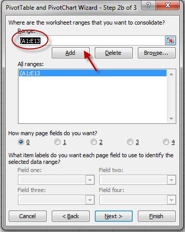
5. In Step 2b, specify a summary table range in the Range field (A1:E13 for the sample data) and click Add; click Next to move on to Step 3.
6. In Step 3, select a location for the pivot table and click the Finish button. Excel creates a pivot table from the data and displays the PivotTable Field list.
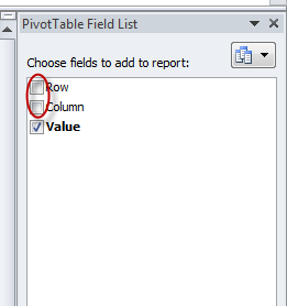
7. In the PivotTable Field List, deselect the check boxes from the fields named Row and Column.
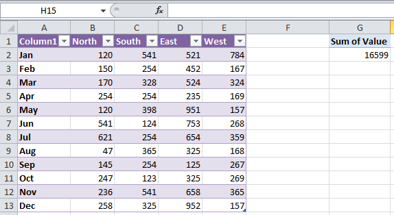
This leaves the pivot table with only a data field: Sum of Value. At this point, a small pivot table shows only the sum of all values (see Figure 167-2).
Figure 167-2: This small pivot table can be expanded.
To finish up, double-click the cell that contains the total (17147, in this example). Excel creates a new sheet that displays the original data in the form of a table. Figure 167-3 shows part of this 48-row table.
The column headings display generic descriptions (Row, Column, and Value), so you probably want to change these headings to make them more descriptive.
Figure 167-3: The summary table has been successfully converted to a table.
