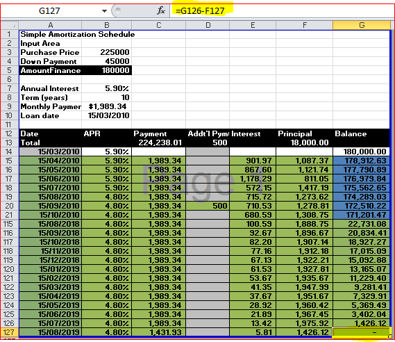
A dynamic amortization schedule
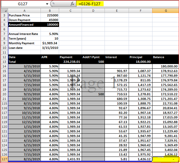
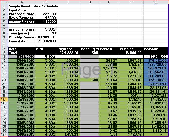
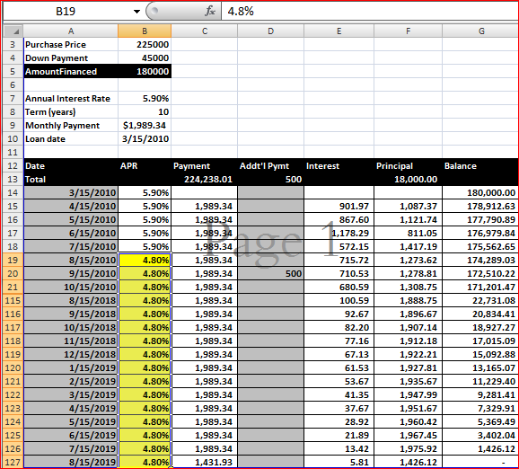
The example in this section builds on the previous example. Figure 13-2 shows a loan amortization schedule that allows the user to define input parameters beyond the amount, rate, and term. Notice that rows 22 through 114 are hidden.
Figure 13-2: A dynamic amortization schedule.
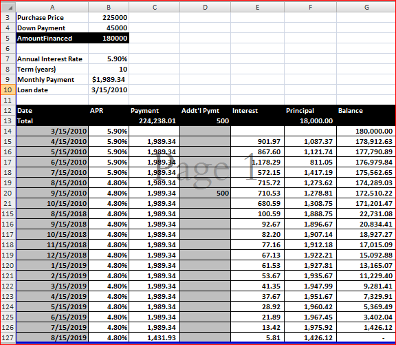
The first difference you’ll notice is that this schedule has more shaded cells, meaning there are more cells that the user can change. Also, a column has been added for the annual percentage rate, which now can be different for every period.
User input section
Not much has changed in Input Area at the top. The interest rate is labeled Starting Rate, and the payment is labeled Computed Payment, indicating that they are subject to change.
Summary information
The user can now change the term; the interest rates; and the payments, which can and usually will change the maturity date. For the summary information, you want to sum only the relevant rows. The formula in C13 is
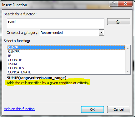
=SUMIF($G15:$G374,”>=0”,C15:C374)
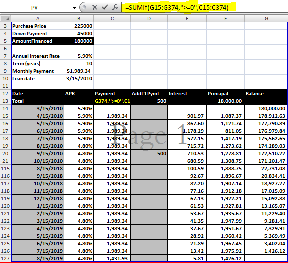
After the Balance in column G is zero, the amortization is complete. This SUMIF function sums only those payments up until that point. This formula is copied across to the interest and principal columns, and the absolute column reference ensures the new formulas still point to column G.
With so many user changeable fields in the schedule, many of the formulas have to change to account for different conditions. An amortization schedule has two kinds of user input data:
-Data that changes for one payment only
-Data that changes for all subsequent payments
When the interest rate changes for one payment, it changes for all subsequent payments — at least, until it changes again. It doesn’t go back to the old rate. For that reason, the APR column relies on the data directly above it. The formula in B15 pulls the starting interest rate from the user input section. This formula, in B16 and copied down, simply repeats the previous month’s rate: =B15
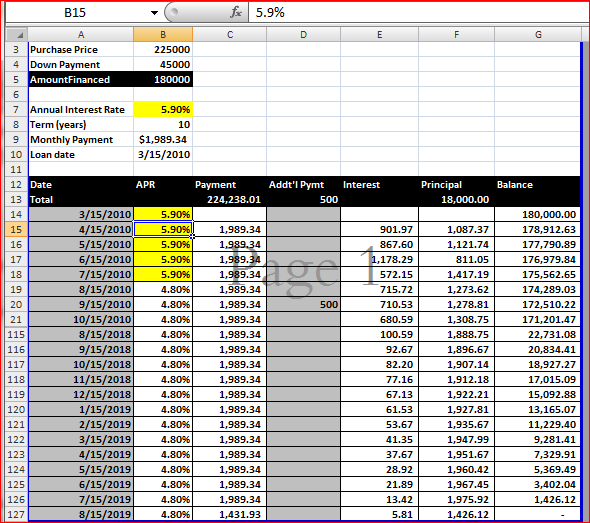
This allows the user to enter a new rate when it changes and have that rate continue down until it’s manually changed again. In this example, the bank informed you that the rate was reduced to 4.8% for the fifth payment (row 19). That rate was entered in B19, and all rates after that reflect the change.
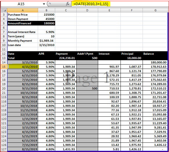
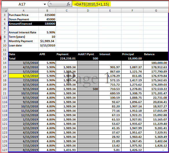
The payment date is an example of data that changes for one payment. If a payment is made late, it doesn’t mean that all subsequent payments will be late. In this example, the third payment (row 17) was made ten days late. This had no effect on the next month’s payment, which was made on time. For this type of data, the increments need to be made against a base that doesn’t change. The formula in A15 is
=DATE(YEAR(Loan_Date),MONTH(Loan_Date)+ROW()–14,DAY(Loan_Date))
This formula is copied down to all the rows. Unlike the previous example, it doesn’t rely on the date above it. Rather, it uses the Loan_Date range as its base. Because the payments start in row 15, the current row less 14 is used to increment the month.
The point of these formulas is to allow the user to overwrite the formula with a literal date value and not affect the rest of the dates. In cell A17, the user replaced the formula by entering a new date, which changed the calculation for that payment but did not affect future payments.
Because you provide a separate column for an additional payment, the payment should never change — except that it needs to account for any previous rounding errors in the last payment.
The formula in C15 is
=IF(G14+E15–Monthly_Payment–D15<5,G14+E15–D15,Monthly_Payment)
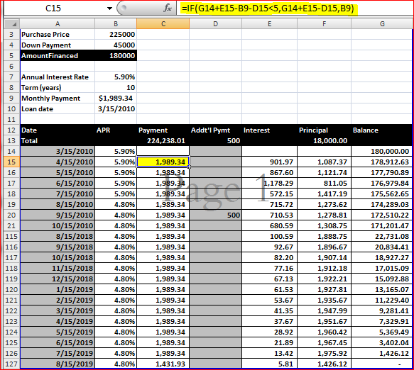
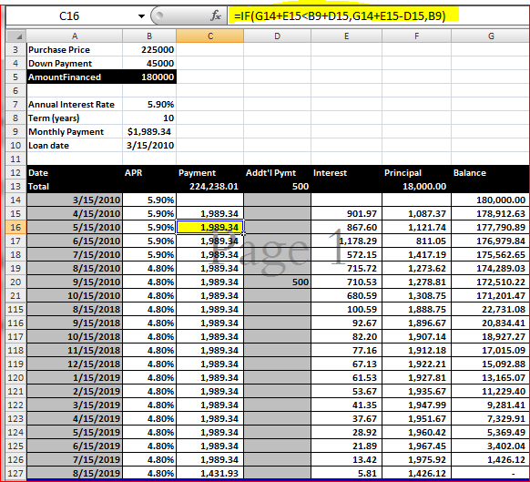
Normally, if the remaining balance is less than the normal payment, just the balance (plus interest) is paid. However, in this example, I don’t want a last payment of less than $5. If a normal payment would leave such a balance, it is just added to the last payment. There’s nothing wrong with a really small final payment. If you don’t mind it, you can simplify the formula to
=IF(G14+E15<Monthly_Payment+D15,G14+E15–D15,Monthly_Payment)
The interest calculation now has to account for the fact that the user may make a payment early or late. Instead of dividing the rate by 12, as in the last example, the rate is multiplied by a ratio of the number of days outstanding to 365. The formula in E15 is
=ROUND(G14*B15*(A15–A14)/365,2)
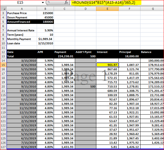
The principal column calculation is similar to the previous example except that any additional payment must be added in. The formula in F15 is
=C15+D15–E15
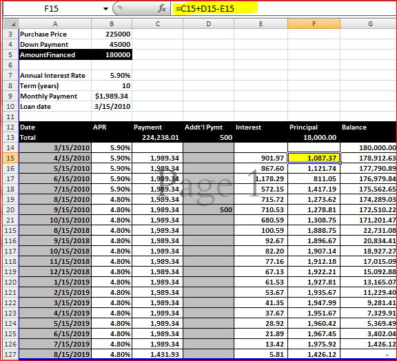
The balance is computed by subtracting the principal portion of the current payment from the previous balance, exactly as it was in the previous example.
Finishing touches
As you can see in Figure 13-2 (which hides rows in the middle so you can see the last payment), the final payment is represented in row 127, and there are no calculations below that. I didn’t just guess right, however. All the cells in the schedule, starting in row 15, have conditional formatting applied to them. If column G of the row above is zero or less, both the background color and the font color are white, rendering them invisible.
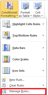
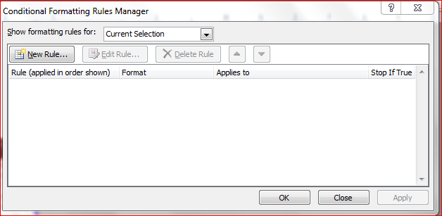
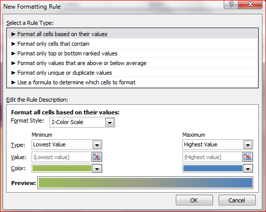
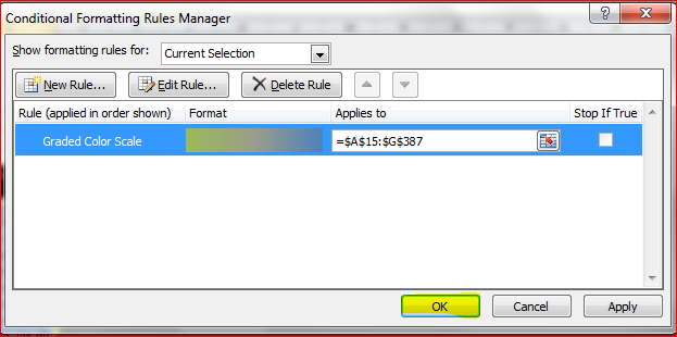
To apply conditional formatting, select the range A15:G374 and choose the Home➜Styles➜ Conditional Formatting command. Add a formula rule with this formula: =$G14<=0
The absolute column means that every column in the selection will refer to column G; the relative row means the row applies to the row above, regardless of which row you’re in.
For more information on conditional formatting, refer to Chapter 19.
The formulas are present in a row beyond row 127 (they exist for up to 360 months), but they are hidden using conditional formatting to make the table size dynamic as well.
